40 move data labels excel
A Step by Step Guide on How to Sort Data in Excel Select the dataset > Click on the Sort option in the Data tab. Choose the Area column to sort. Under Sort On, select Cell Values. Under Order, choose the Custom List. Fig: Custom Sort list In the Custom Lists dialog box, add the List entries separated by commas - S. County, Central, N. County. Click on Add > Select Ok. How to Use Excel Pivot Table Label Filters Right-click on an item in the Row Labels or Column Labels In the pop-up menu, click Filter, then click Hide Selected Items. The item is immediately hidden in the pivot table. Quickly Hide All But a Few Items You can use a similar technique to hide most of the items in the Row Labels or Column Labels.
Excel help? - Microsoft Tech Community Labels: Excel 144 Views . 0 Likes ... Unless there are reasons why the Table has to stay at the top of the sheet, you could simply move it down a few rows to make room for the supplementary calculation. 0 Likes . Reply. ... The main problem could be that I use defined Names rather than cell references to refer to data. From the picture it seems ...
Move data labels excel
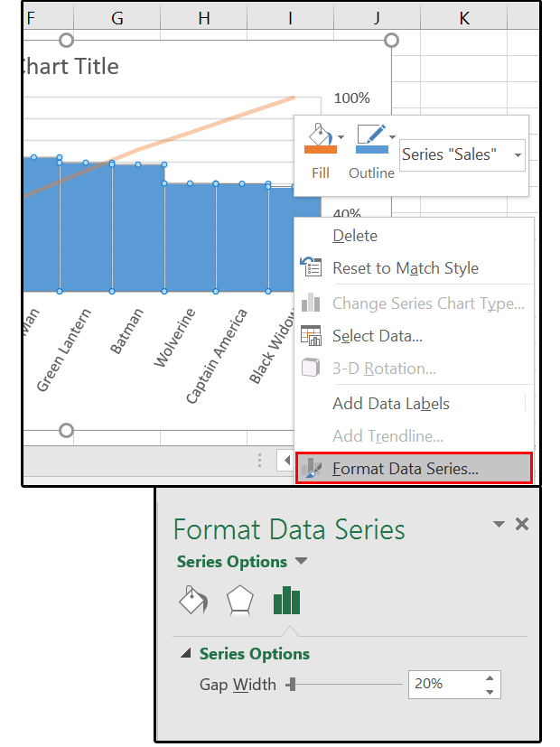
How to Freeze Header Rows or Columns in Excel On the Freeze Panes button, click the small triangle in the lower right corner. You should see a new menu with your 3 options. Click the option Freeze Panes. Scroll down your worksheet to make sure the first row stays at the top. Scroll across your sheet to make sure your first column stays locked on the left. How to add secondary axis in Excel (2 easy ways) - ExcelDemy Right click on the data series => Choose the Format Data Series option from the menu => Format Data Series task pane appears => Select Fill & Line tab => Choose Marker => Marker Options => Select Built-in => Using Type and Size drop down, choose preferred Marker and change the Size of the marker. Excel cells turning white - Microsoft Community Excel cells turning white. Whenever I enter a data, formula, or text in a cell on Excel, the entire row of that cell turns white when pressed Enter. Not sure why this is happening. If scrolling down the Excel sheet, I noticed more and more cells and rows are white. When I switch to a different app, some data of the cells are now visible and not ...
Move data labels excel. Importing Data into SPSS - LibGuides at Kent State University Once the data in your Excel file is formatted properly it can be imported into SPSS by following these steps: Click File > Open > Data. The Open Data window will appear. In the Files of type list select Excel (*.xls, *.xlsx, *.xlsm) to specify that your data are in an Excel file. How to Use Slicers in Excel to Easily Filter your Pivot Tables This is where Slicers come in. Go to the PivotTable Analyze tab and click on Insert Slicer. A menu will pop up where you can select the parameters you want to slice your data set. Select TERRITORY,... what is a stacked bar chart? — storytelling with data If you're using Excel, a good value for the spacing between bars is somewhere between 30% and 35%. Intentionally set the order of your bars by maintaining the inherent order of the data, or arranging the bars from biggest to smallest. Move data labels inside the ends of bars. Don't truncate the length of the bars. How to Make a Data Table for What-If Analysis in Excel Go to the Data tab, click the What-If Analysis drop-down arrow, and pick "Data Table.". In the Data Table box that opens, enter the cell reference for the changing variable and per your setup. For our example, we enter the cell reference B3 for the changing interest rate in the Column Input Cell field. Again, we're using a column-based ...
How to Create Excel Pivot Table (Includes practice file) You can also move or "pivot" your data by right-clicking a data field on the table and selecting the " Move " menu. From here, you can move a column to a row or even change the position. An example of this might be the "LAST VOTED" values since Excel will sort by the month first. SPSS Tutorials: Recoding String Variables (Automatic Recode) Click Transform > Automatic Recode. Double-click variable State in the left column to move it to the Variable -> New Name box. Enter a name for the new, recoded variable in the New Name field, then click Add New Name. Check the box for Treat blank string values as user-missing. Click OK to finish. How to Automate an Excel Sheet in Python? - GeeksforGeeks Write down the code given below. wb returns the object and with this object, we are accessing Sheet1 from the workbook. wb = xl.load_workbook ('python-spreadsheet.xlsx') sheet = wb ['Sheet1'] Step 3. To access the entries from rows 2 to 4 in the third column (entry for price column) we need to add a for loop in it. Learn about the default labels and policies to protect your data ... Activate the default labels and policies. To get these preconfigured labels and policies: From the Microsoft Purview compliance portal, select Solutions > Information protection. If you don't immediately see this option, first select Show all from the navigation pane.. If you are eligible for the Microsoft Purview Information Protection default labels and policies, you'll see the following ...
Excel's data from picture now in Windows! - Office Watch Data from Picture. Excel's Data from Picture is tucked away on the Data tab among all the Get & Transform Data options. Select a photo or use the one in the clipboard. It will appear in a Data from Picture side-pane after a short pause as it's uploaded to Microsoft's servers and analyzed. Below the image is the returned data in cells. Create Radial Bar Chart in Excel - Step by step Tutorial Prepare the labels for the radial bar chart. First, create a helper column for the data labels on column E. Then enter the formula =B12&" ("&C12&")" on cell E12. You can use the CONCATENATE function also. Finally, fill down the formula for "E12:E16". Go to the Ribbon, and click on the Insert tab. Insert a Text box. Importing data into Pipedrive with spreadsheets - Knowledge Base Once you understand how Pipedrive data works and formatted your spreadsheet properly, you can start your import. Step 1: Upload your file. Go to " ... " (More)> Import data > From a spreadsheet. Click "Upload file" and select the file that you intend to import. Pipedrive supports Excel (.xls and .xlsx) and .csv files. improve your graphs, charts and data visualizations — storytelling with ... If you're using Excel, a good value for the spacing between bars is somewhere between 30% and 35%. Intentionally set the order of your bars by maintaining the inherent order of the data, or arranging the bars from biggest to smallest. Move data labels inside the ends of bars. Don't truncate the length of the bars.
Диаграммы Excel - элементы диаграммы - CoderLessons.com
How to Make an Excel Box Plot Chart - Contextures Excel Tips Copy the cells with the Average label, and the formulas Click on the chart, and on the Ribbon's Home tab, click the arrow on the Paste button Click Paste Special. In the Paste Special dialog box, choose "New Series", Values in Rows, and "Series Names in First Column", and click OK

Restructuring (Normalizing) data for Pivot tables using Pivot tables - How To - PakAccountants.com
Learn about sensitivity labels - Microsoft Purview (compliance) To reorder the label policies, select a sensitivity label policy > choose the ellipsis on the right > Move down or Move up. Note Remember: When there is a conflict of settings for a user who has multiple policies assigned, the setting from the policy with the highest priority (lowest position) is applied.

Directly Labeling Excel Charts - PolicyViz
Linear Regression Excel: Step-by-Step Instructions Charting a Regression in Excel. We can chart a regression in Excel by highlighting the data and charting it as a scatter plot. To add a regression line, choose "Layout" from the "Chart Tools" menu ...
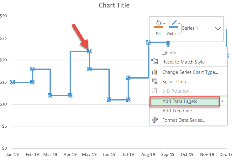
How to Create a Step Chart in Excel - Automate Excel
Questions from Tableau Training: Can I Move Mark Labels? This brings us to label-positioning tactic #2 (from above): "Click directly on the mark and set it free to be wherever you choose." This method is as simple as clicking on the label you want to reposition — wait until you get the following cross quadruple arrow cursor (at least that's what I call it): Then, drag the label wherever you want.
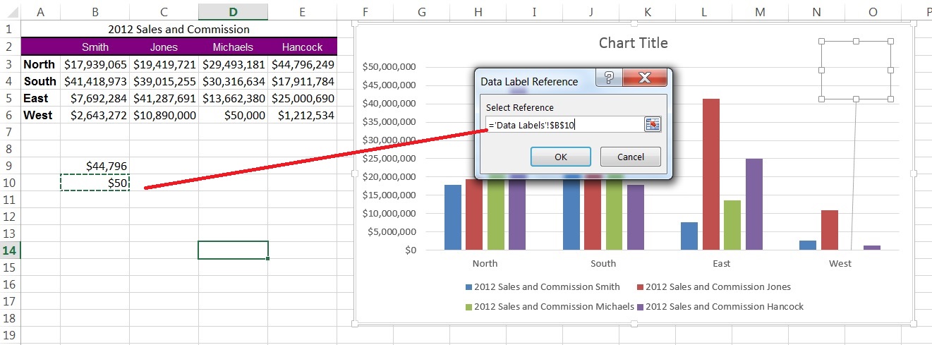
Quick Tip: Excel 2013 offers flexible data labels - TechRepublic
50 Excel Shortcuts That You Should Know in 2022 - Simplilearn Alt + Shift + Left arrow. Now that we have looked at the different shortcut keys for formatting cells, rows, and columns, it is time to jump into understanding an advanced topic in Excel, i.e. dealing with pivot tables. Let's look at the different shortcuts to summarize your data using a pivot table.

30 Label The Excel Window - Labels Design Ideas 2020
linkedin-skill-assessments-quizzes/microsoft-excel-quiz.md at ... - GitHub In the Data tab, click the Sort button. Add two levels to the default level. Populate the Sort-by fields in this order: Group, Last Name, First Name. C; Highlight the entire dataset. In the Data tab, click the Sort button. The headers appear. Drag the headers into this order: Group, Last Name, First Name. D; Select a cell in the Group column, then sort.

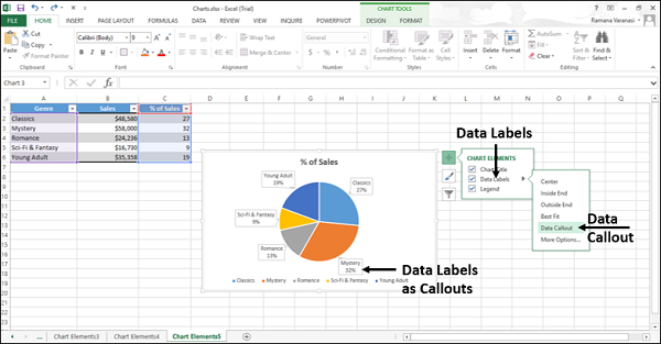
410 How to display percentage labels in pie chart in Excel 2016 - YouTube
Excel IF function with multiple conditions - Ablebits.com Advanced Excel IF formula examples: multiple AND/OR criteria, nested IF statements, array formulas and more. ... For powerful data analysis, however, you may often need to evaluate multiple conditions at a time. The below formula examples will show you the most effective ways to do this. ... To have both labels in one column, nest the above ...
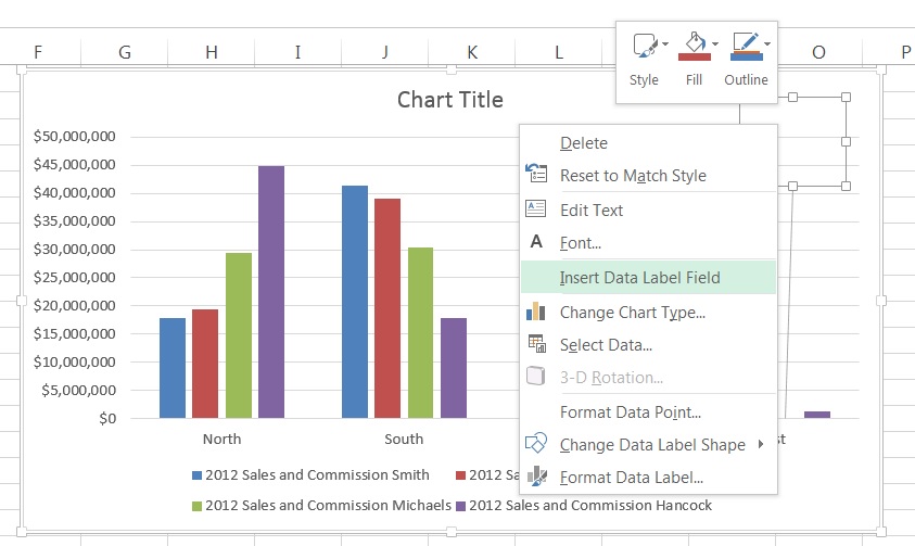
Quick Tip: Excel 2013 offers flexible data labels - TechRepublic
Unlink Chart Data - Peltier Tech =SERIES('C:\Long Path[Data Source.xlsx]Sheet1'!$C$2,'C:\Long Path[Data Source.xlsx]Sheet1'!$B$3:$B$8,'C:\Long Path[Data Source.xlsx]Sheet1'!$C$3:$C$8,1) Copy a Picture of the Chart One way to represent an unlinked chart is to copy a picture of the chart, then paste it where desired.
Stock Investment Tracker | Stock Investment Performance Tracker
How to Create Professional Charts in Excel | by Dobromir Dikov, FCCA ... Open the Format Data Labels menu, pick a better position for the labels, and in the Number options, format the number with the formatting code #,###, "k". This format string will show the values in...

Building a BumpChart in Excel (with VBA) - PolicyViz
Excel cells turning white - Microsoft Community Excel cells turning white. Whenever I enter a data, formula, or text in a cell on Excel, the entire row of that cell turns white when pressed Enter. Not sure why this is happening. If scrolling down the Excel sheet, I noticed more and more cells and rows are white. When I switch to a different app, some data of the cells are now visible and not ...

SQL & BI Learning: Pie Chart with data labels outside in ssrs
How to add secondary axis in Excel (2 easy ways) - ExcelDemy Right click on the data series => Choose the Format Data Series option from the menu => Format Data Series task pane appears => Select Fill & Line tab => Choose Marker => Marker Options => Select Built-in => Using Type and Size drop down, choose preferred Marker and change the Size of the marker.

Adobe Acrobat Standard Help 7.0 Instruction Manual 7 En
How to Freeze Header Rows or Columns in Excel On the Freeze Panes button, click the small triangle in the lower right corner. You should see a new menu with your 3 options. Click the option Freeze Panes. Scroll down your worksheet to make sure the first row stays at the top. Scroll across your sheet to make sure your first column stays locked on the left.

Enable or Disable Excel Data Labels at the click of a button - How To - PakAccountants.com
Worth Data UK - LabelRIGHT Ultimate Bar Code Printing & Design Software for Windows

Excel 2010 Change the Positions of Data Labels Automatically - YouTube

Enable or Disable Excel Data Labels at the click of a button - How To - PakAccountants.com
Excel 2016 charts: How to use the new Pareto, Histogram, and Waterfall formats | PCWorld
Post a Comment for "40 move data labels excel"